Climate Vulnerability in Malawi
Replication of: Vulnerability modeling for sub-Saharan Africa
Original study by Malcomb, D. W., E. A. Weaver, and A. R. Krakowka. 2014. Vulnerability modeling for sub-Saharan Africa: An operationalized approach in Malawi. Applied Geography 48:17–30. DOI:10.1016/j.apgeog.2014.01.004
Replication Authors: Maja Cannavo, Joseph Holler, Kufre Udoh, Open Source GIScience students of fall 2019 and Spring 2021
Special thanks to my group members--we all worked together to write our workflow and data sources section:
Drew An-Pham
Emma Clinton
Jacob Freedman
Nick Nonnenmacher
Alitzel Villaneuva
Also many thanks to Vincent Falardeau for invaluable help with mapping in ggplot, specifically getting the legend items properly ordered in Figure 2 and using a diverging color ramp in Figure 4.
Replication Materials Available at: majacannavo/RP-Malcomb
Created: 14 April 2021 |
Revised: 25 May 2021
Abstract
The original study is a multi-criteria analysis of vulnerability to Climate Change in Malawi, and is one of the earliest sub-national geographic models of climate change vulnerability for an African country. The study aims to be replicable, and had 40 citations in Google Scholar as of April 8, 2021.
Original Study Information
The study region is the country of Malawi. The spatial support of input data includes DHS survey points, Traditional Authority boundaries, and raster grids of flood risk (0.833 degree resolution) and drought exposure (0.416 degree resolution).
The original study was published without data or code, but has detailed narrative description of the methodology. The methods used are feasible for undergraduate students to implement following completion of one introductory GIS course. The study states that its data are available for replication in 23 African countries.
Data Description and Variables (compiled as a group)
Assets & Access
Source: The DHS Program—Data. (2010). The DHS Program--USAID. Retrieved April 19, 2021, from https://dhsprogram.com/Data/
Collected by trained USAID staff using GPS receivers. GPS readings correspond to center of household cluster (one randomized point per household cluster).
In this analysis, we use the variables listed in Table 1 to determine the average adaptive capacity of each TA area. Data transformations are outlined below.
Table 1. Variables used in calculating adaptive capacity.
| Variable Code | Definition |
|---|---|
| HHID | "Case Identification" |
| HV001 | "Cluster number" |
| HV002 | Household number |
| HV246A | "Cattle own" |
| HV246D | "Goats own" |
| HV246E | "Sheep own" |
| HV246G | "Pigs own" |
| HV248 | "Number of sick people 18-59" |
| HV245 | "Hectares for agricultural land" |
| HV271 | "Wealth index factor score (5 decimals)" |
| HV251 | "Number of orphans and vulnerable children" |
| HV207 | “Has Radio” |
| HV243A | “Has a Mobile Telephone” |
| HV219 | "Sex of Head of Household” |
| HV226 | “Type of Cooking Fuel” |
| HV206 | "Has electricity” |
| HV204 | “Time to get to Water Source” |
Transformations:
- Eliminate households with null and/or missing values
- Join TA and LHZ ID data to the DHS clusters
- Pre-process the livestock data:
- Eliminate NA values for livestock
- Sum counts of all different kinds of livestock into a single variable
- Normalize each indicator variable and rescale from 1-5 (real numbers) based on percent rank
- Apply weights to normalized indicator variables to get scores for each category (assets, access)
- Find the stats of the capacity of each TA (min, max, mean, std. dev.)
- Join ta_capacity to TA based on ta_id
- Prepare breaks for mapping
- Class intervals based on capacity_2010 field
- Take the values and round them to 2 decimal places
- Put data in 4 classes based on break values
Demographic and Health Survey data are a product of the United States Agency for International Development (USAID). Variables contained in this dataset are used to represent adaptive capacity (access + assets) in the Malcomb et al.’s (2014) study. These data come from survey questionnaires with large sample sizes. The DHS data used in our study were collected in 2010. In Malawi, the provenance of the DHA data dates back as far as 1992, but has not been collected consistently every year. Each point in the household dataset represents a cluster of households with each cluster corresponding to some form of census enumeration units, such as villages in rural areas or city blocks in urban areas DHS GPS Manual. This means that each household in each cluster has the same GPS data. However, the GPS point for each cluster is given a random offset in the interest of protecting privacy, so the coordinates are not precise.
Missing data is a common occurrence in this dataset as a result of negligence or incorrect naming. However, according to the DHS GPS Manual, these issues are easily rectified and data are typically recollected for sites where they are missing. Sometimes, however, missing information is coded in as such or assigned a proxy location. The DHS website acknowledges the high potential for inconsistent or incomplete data in such broad and expansive survey sets. Missing survey data (responses) are never estimated or made up; they are instead coded as a special response indicating the absence of data. As well, there are clear policies in place to ensure the data’s accuracy. More information about data validity can be found on the DHS’s Data Quality and Use site.
Malawi Traditional Authorities:
Source: Download GADM data (version 2.8). (2018). Database of Global Administrative Areas. https://gadm.org/download_country_v2.html
Major Lakes:
Source: http://www.masdap.mw/ Taken from OSM
Transformations: used in EA variable to classify major lakes as such in final representation
Livelihood Zones
The Livelihood Zones data is created by aggregating general regions where similar crops are grown and similar ecological patterns exist. This data exists originally at the household level and was aggregated into Livelihood Zones. To construct the aggregation used for “Livelihood Sensitivity” in this analysis, we use these household points from the FEWSNET data that had previously been aggregated into livelihood zones. The four Livelihood Sensitivity categories are 1) Percent of food from own farm (6%); 2) Percent of income from wage labor (6%); 3) Percent of income from cash crops (4%); and 4) Disaster coping strategy (4%). In the original R script, household data from the DHS survey was used as a proxy for the specific data points in the livelihood sensitivity analysis (transformation: Join with DHS clusters to apply LHZ FNID variables). With this additional FEWSNET data at the household level, we can construct these four livelihood sensitivity categories using existing variables (Table 2). The LHZ data variables are outlined in Table 2. The four categories used to determine livelihood sensitivity were ranked from 1-5 based on percent rank values and then weighted using values taken from Malcomb et al. (2014).
Table 2: Constructing livelihood sensitivity categories
| Livelihood Sensitivity Category (LSC) | Percent Contributing | How LSC was constructed |
|---|---|---|
| Percent of food from own farm | 6% | Sources of food: crops + livestock |
| Percent of income from wage labor | 6% | Sources of cash: labour etc. / total * 100 |
| Percent of income from cash crops | 4% | sources of cash (Crops): (tobacco + sugar + tea + coffee) + / total sources of cash * 100 |
| Disaster coping strategy | 4% | Self-employment & small business and trade: (firewood + sale of wild food + grass + mats + charcoal) / total sources of cash * 100 |
Source: Download https://fews.net/data_portal_download/download?data_file_path=http%3A//shapefiles.fews.net.s3.amazonaws.com/LHZ/MW_LHZ_2009.zip
Sources: Malawi Baseline Livelihood Profiles, Version 1* (September 2005). Made by Malawi National Vulnerability Assessment Committee in collaboration with the SADC FANR Vulnerability Assessment Committee -- file in metadata called mw_baseline_rural_en_2005.pdf
Variables
17 livelihood zones
Livelihood zones created through: “The approach is to identify those factors (such as climate, soil, proximity to rivers, access to markets etc.) that determine the basic food and income options (the crops that will grow, the livestock that can be raised, the wild plants that can be collected, the fish that can be caught, and so on) and then to group similar areas together. In the case of Malawi, the exercise was one of updating an earlier food economy zone map prepared by Save the Children dating from 1996.” (2)
The data we used is just to extract the geometries of the livelihood zone data and basically create the geometry boundaries of Malawi for processing to determine park boundaries
FEWSNET data:
- Percent of food from own farm (6%)
- Percent of income from wage labor (6%)
- Payment in cash: labour, employment, and remittances
- Percent of income from cash crops (4%)
- Crop = tobacco-burley, tobacco-oriental, cotton, sugar cane, maize, tea, coffee
- Disaster coping strategy (4%)
- Percent of cash sourced from self-employment & small business and trade: (firewood + sale of wild food + grass + mats + charcoal)
Transformations:
- Join with DHS clusters to apply LHZ FNID variables
- Clip TA boundaries to Malawi (st_buffer of LHZ to .01 m)
- Create ecological areas: LHZ boundaries intersected with TA boundaries to clip out park/conservation boundaries and rename those park areas with the park information from TA data), combined with lake data to remove environmental areas from the analysis
Physical Exposure
Floods
Dataset title: “Global estimated risk index for flood hazard”
“This dataset includes an estimate of the global risk induced by flood hazard. Unit is estimated risk index from 1 (low) to 5 (extreme). This product was designed by UNEP/GRID-Europe for the Global Assessment Report on Risk Reduction (GAR). It was modeled using global data. Credit: UNEP/GRID-Europe.” This dataset stems from work collected by multiple agencies and funneled into the PREVIEW Global Risk Data Platform, “an effort to share spatial information on global risk from natural hazards.” The dataset was designed by UNEP/GRID-Europe for the Global Assessment Report on Risk Reduction (GAR), using global data. A flood estimation value is assigned via an index of 1 (low) to 5 (extreme). The data use the WGS 1984 datum, span the years 1999-2007, and are reported in raster format with spatial resolution 1/24 degree x 1/24 degree.
Droughts
Dataset title: "Physical exposition to droughts events 1980-2001"
This dataset uses the Standardized Precipitation Index to measure annual drought exposure across the globe. The Standardized Precipitation Index draws on data from a “global monthly gridded precipitation dataset” from the University of East Anglia’s Climatic Research Unit, and was modeled in GIS using methodology from Brad Lyon at Columbia University. The dataset draws on 2010 population information from the LandScanTM Global Population Database at the Oak Ridge National Laboratory. Drought exposure is reported as the expected average annual (2010) population exposed. The data were compiled by UNEP/GRID-Europe for the Global Assessment Report on Risk Reduction (GAR). The data use the WGS 1984 datum, span the years 1980-2001, and are reported in raster format with spatial resolution 1/24 degree x 1/24 degree.
Sources: UNEP/GRID-Europe
Global Risk Data Platform: Data-Download. (2013). Global Risk Data Platform. https://preview.grid.unep.ch/index.php?preview=data&lang=eng
Drought--Physical exposition to droughts events 1980-2001: https://preview.grid.unep.ch/index.php?preview=data&events=droughts&evcat=4&lang=eng
Global estimated risk index for flood hazard: https://preview.grid.unep.ch/index.php?preview=data&events=floods&evcat=5&lang=eng
Variables:
- Estimated risk for flood hazard
- Exposition to drought events
Transformations
- Load in UNEP raster
- Set CRS for drought to EPSG:4326
- Set CRS for flood to EPSG:4326
- Reproject, clip, and resample based on bounding box (dimensions: xmin = 35.9166666666658188, xmax = 32.6666666666658330, ymin = -9.3333333333336554, ymax = -17.0833333333336270) and resolution of blank raster we created: resolution is 1/24 degree x 1/24 degree
- Use bilinear resampling for drought to average continuous population exposure values
- Use nearest-neighbor resampling for flood risk to preserve integer values
Analytical Specification
The original study was conducted using ArcGIS and STATA, but does not state which versions of these software were used. The replication study will use R.
Materials and Procedure (compiled as a group)
Process Adaptive Capacity
- Bring in DHS Data [Households Level] (vector)
- Bring in TA (Traditional Authority) boundaries and LHZ (livelihood zones) data
- Get rid of unsuitable households (eliminate NULL and/or missing values)
- Join TA and LHZ ID data to the DHS clusters
- Pre-process the livestock data
- Filter for NA livestock data
- Update livestock data (summing different kinds)
- FIELD CALCULATOR: Normalize each indicator variable and rescale from 1-5 (real numbers) based on percent rank
- FIELD CALCULATOR / ADD FIELD: Apply weights to normalized indicator variables to get scores for each category (assets, access)
- SUMMARIZE/AGGREGATE: find the stats of the capacity of each TA (min, max, mean, sd)
- Join ta_capacity to TA based on ta_id
- Prepare breaks for mapping
- Class intervals based on capacity_2010 field
- Take the values and round them to 2 decimal places
- Put data in 4 classes based on break values
- Save the adaptive capacity scores
Process Livelihood Sensitivity
- Load LHZ .csv into QGIS
- Join LHZ sensitivity data to LHZ polygon layer
- Import this joined layer into R
- Create livelihood sensitivity score data based on breakdown provided in report (Table 2)
- Multiply by 20 to get a score out of 20
Process Physical Exposure
- Load in UNEP raster
- Set CRS for drought
- Set CRS for flood
- Clean and reproject rasters
- Create a bounding box at extent of Malawi
- Add geometry info and precision (st_as_sfc)
- For Drought: use bilinear to avg continuous population exposure values
- For Flood: use nearest neighbor to preserve integer values
- CLIP the traditional authorities with the LHZs to cut out the lake
- RASTERIZE the ta_capacity data with pixel data corresponding to capacity_2010 field
- RASTERIZE the livelihood sensitivity score with pixel data corresponding to capacity_2010 field
- RASTER CALCULATOR:
- Create a mask
- Reclassify the flood layer (quintiles, currently binary)
- Reclassify the drought values (quantile [from 0 - 1 in intervals of 0.2 =5])
- Add component rasters for final weighted score of drought + flood
Aggregate to create final score:
- Create final vulnerability layer using the following formula:
final = (40 - (adaptive capacity)) * 0.40 + drought * 0.20 + flood * 0.20 + (livelihood sensitivity) * 0.20
Compare results with Malcomb et al.
- Digitize Malcomb et al.'s maps of adaptive capacity and overall vulnerability
- Calculate Spearman's rho between reproduced and original adaptive capacity scores to investigate correlation
- Calculate difference between reproduced and original TA adaptive capacity scores, and display on map
- Calculate difference between reproduced and original overall vulnerability scores
- Make scatterplot of reproduced vs. original vulnerability scores
- Calculate Spearman's rho between reproduced and original vulnerability scores to investigate correlation
- Map difference between reproduced and original vulnerability scores
Replication Results
My adaptive capacity scores by traditional authority (Figure 1) display a relatively strong positive correlation with the adaptive capacity scores calculated by Malcomb et al., with a Spearman's rho value of 0.779. (See Figure 2 for a geographic distribution of difference between my reproduction and the original study.) The p-value is infinitesimal at less than 2.2 x 10^-16, although this means little given that we have a very large sample size. Thus, the original study is relatively well supported by the replication. It would be difficult to achieve a Spearman's rho of very close to 1 considering that we did not compare our replication maps directly to Malcomb et al.'s. Instead, we compared our replication maps to maps we created in QGIS to approximate Malcomb et al.'s results as closely as possible using georeferencing and zonal statistics with a TA polygon layer. No deviations were planned from the original study.
Figure 1. Adaptive capacity scores by traditional authority, 2010. (analogous to Malcomb et al. Fig. 4)
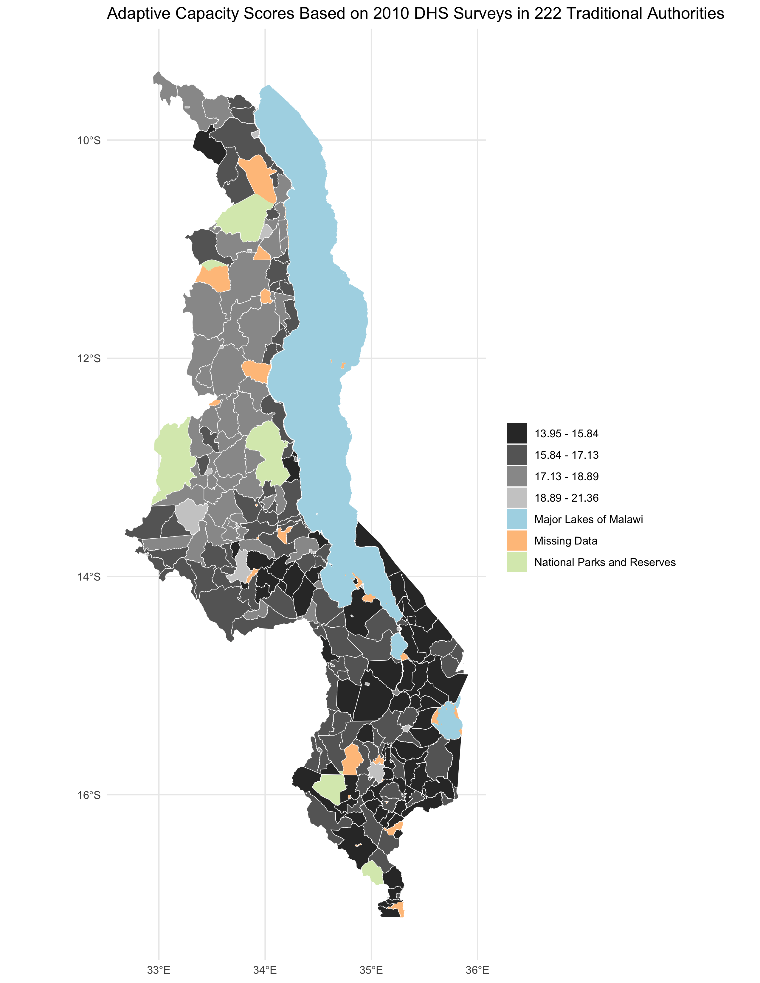
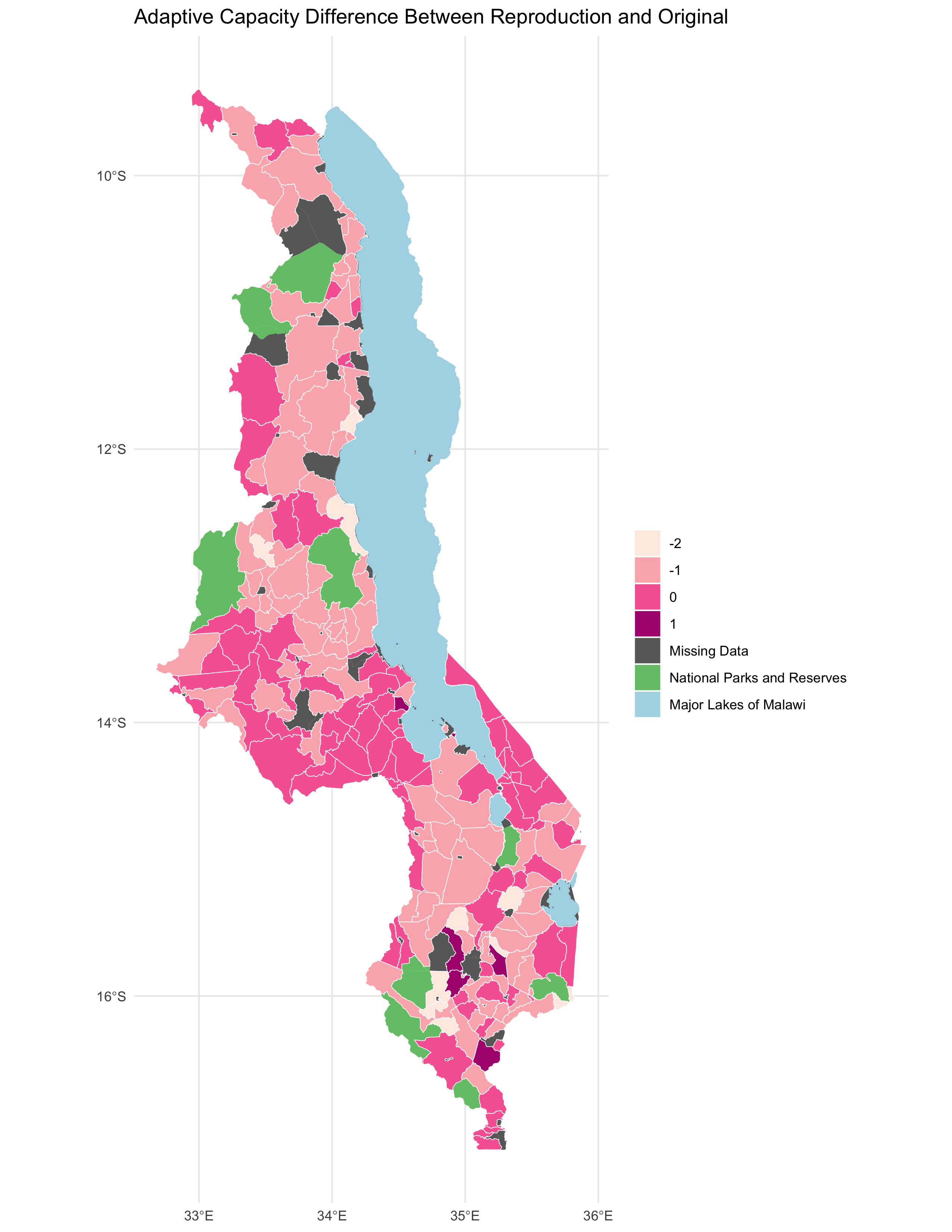
Figure 2. Adaptive capacity difference between reproduction and original.
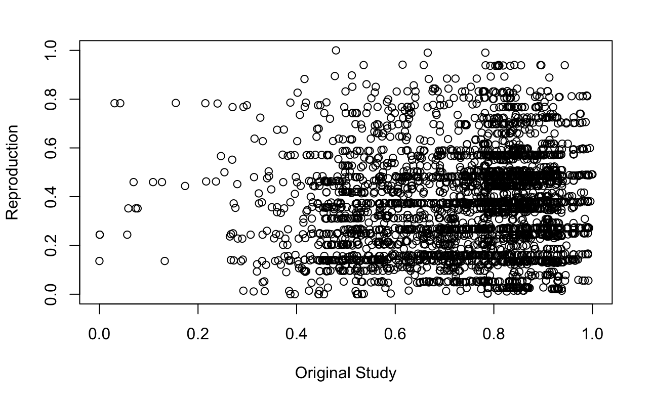
My map of vulnerability to climate change across Malawi (Figure 3) displays a much weaker positive correlation than do my adaptive capacity scores when compared to Malcomb et al.'s results. In this case, Spearman's rho is only 0.114, demonstrating a very weak positive correlation. (See Figure 4 for a geographic distribution of difference between the reproduction and the original. See Figure 5 for a scatterplot point comparison between the results of the original study and the reproduction.) Again, the p-value is very small at 1.49 x 10^-12, but again this is not particularly important as the sample size is so large. This weak correlation is relatively unsurprising given that Malcomb et al.'s description of their methods is ambiguous in many places and leaves significant room for interpretation. We had to determine how exactly to normalize the various variables, as well as how to use the livelihood zones data to develop the variables of percent of food from own farm, percent income from wage labor, percent income from cash crops, and disaster coping strategy. As a result, it is very likely that our scores differ greatly from Malcomb et al.'s, and we must conclude that the results of our reproduction do not support those of the original study.
Figure 3. Vulnerability to Climate Change in Malawi. (analogous to Malcomb et al. Fig. 5)
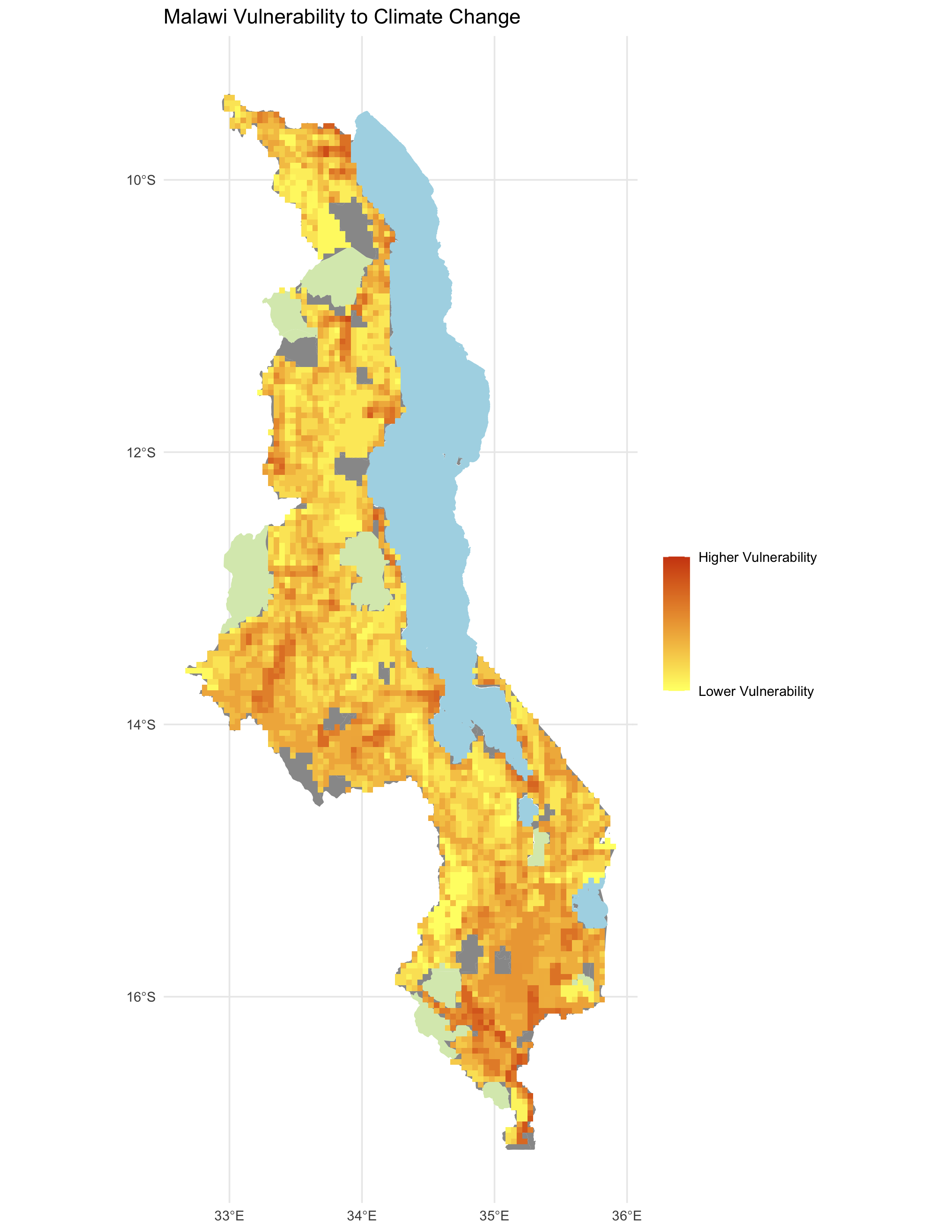
Figure 4. Map of vulnerability difference between reproduction and original.
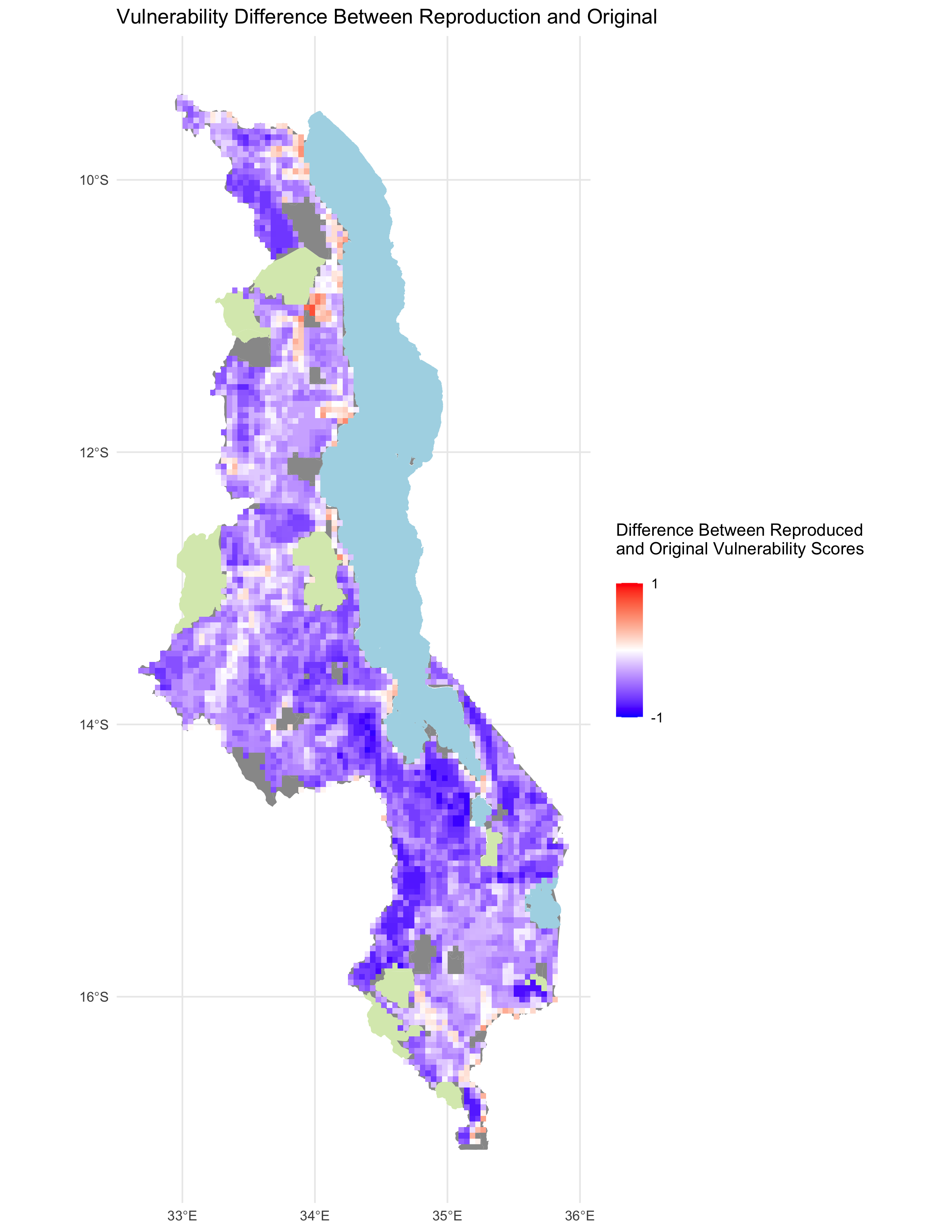
Figure 5. Scatterplot of vulnerability difference between reproduction and original.
Unplanned Deviations from the Protocol
Our group's original workflow based on an initial reading of the paper was relatively rough; we included little detail as to how exactly the data were to be cleaned and the variables calculated. Also, lacking the data, we were unsure of the variables we would have access to, as well as the scale of these variables. For instance, our initial impression was that the DHS data would come at the household level and that further steps would be necessary to aggregate the households into villages and then to aggregate the villages into TAs. Upon gaining access to the code and the data, we realized that the DHS data came in the units of household clusters, so aggregating them into villages would be unnecessary. With access to the data and the code, we were also able to draft a more detailed workflow including elements such as how to normalize the variables to scale them from 1-5, how to resample the flood and drought exposure rasters, and how to mask and rescale the rasters so that their values could eventually be added to achieve the final vulnerability score.
Overall, it proved quite challenging to piece together the general pattern of the workflow prior to accessing the data and code, but upon viewing the data and the R script, the details of the workflow became much clearer. It was also somewhat unclear initially what the LHZ data would look like, so we wrote the part of the workflow relating to these data only after we obtained access to them. Examining the surveys, we could define how to compose and normalize the four livelihood sensitivity indicator variables, as well as how to integrate the livelihood sensitivity scores into the final raster algebra step to calculate the final vulnerability score.
Discussion
While TA adaptive capacity scores display a strong positive correlation between the original study and the reproduction, the same is not true for overall household resilience score. As shown in Figure 2, in the case of many TAs the reproduction and original yielded adaptive capacity scores in the same class (each score was assigned to one of four classes based on a Jenks classification), and in most other case the difference in classes was minimal (1 or -1). In only a few cases did the two results differ by more than 1. The Spearman's rho value of 0.779 serves to reinforce the conclusion that the adaptive capacity score distributions of the original study and the replication mirror each other closely.
It is relatively unsurprising that the adaptive capacity scores from the two studies match each other so well. The original and reproduction both draw from the same dataset and use concrete variables, most of which can be taken directly from the DHS survey data, so little interpretation is required as to how to derive them. Moreover, since the adaptive capacity scores are visualized in four classes using a Jenks classification, the actual numerical scores are not nearly as important as their distribution. At one point in the workflow, we had to decide whether or not to multiply each adaptive capacity score by 20, as Joseph Holler and Kufre Udoh did in their replication of the study to bring their scores closer to those of the original analysis. I chose not to include this step, since I saw no concrete reason to, and as a result my adaptive capacity scores were numerically much smaller than they would have been otherwise. However, this did not impede my classification from mapping closely to Malcomb et al.'s, since multiplying by 20 would not have affected the distribution of my scores.
Nevertheless, this decision not to multiply by 20 may have been part of the reason why my results display such a weak correlation with those of Malcomb et al. in terms of overall vulnerability score. By choosing not to multiply by 20, I significantly decreased the weight of adaptive capacity in my final household resilience calculation. As a result, I would imagine that my overall vulnerability score does not assign nearly a large enough weight to adaptive capacity in comparison to livelihood sensitivity and physical exposure. Adaptive capacity still ends up being a score out of 40, but this score does not vary much according to variations in actual adaptive capacity since the score out of 40 is calculated as 40 - (previously calculated adaptive capacity).
Another major contributor to the disparity in overall vulnerability score is probably differences between how my group calculated livelihood sensitivity and how Malcomb et al. did so. Although the authors of the original study describe the indicator variables they used to compute livelihood sensitivity, they fail to give an explicit definition of which fields in the LHZ data they used to derive each variable, most conspicuously disaster coping strategy (Malcomb et al. 2014, p. 21). As a result, we had to use our best judgment interpreting the authors' descriptions, but our choices likely diverged from theirs. As Tate (2013) argues, "[u]ncertainty in social vulnerability indexes stems from modeling decisions made during their development," which "is largely a sequential process" (p. 528). Uncertainty can arise from choices in the indicator variables used, as well as how they are transformed, normalized, weighted, and aggregated, among other factors (Tate 2013, p. 528). The uncertainty embedded in Malcomb et al.'s analysis throughout these processes is reflected in the failure of this reproduction to approach the original authors' results. Ultimately, a dearth of methodological details and lack of source code made a fully successful reproduction of this analysis very difficult.
Conclusion
Ultimately, this analysis was partly successful in reproducing Malcomb et al.'s study of climate change vulnerability in Malawi. We found that it was much easier to reliably reproduce results for the parts of the study where indicator variables were clearly delineated and it was readily apparent how data points mapped to these variables. This reproduction also lends support to Tate's (2013) conceptualization of vulnerability index development as "a sequential process" wherein uncertainty arising at each step has an effect on each step further down the line until the final result is computed (p. 528). I was able to achieve a fairly successful replication of Malcomb et al.'s adaptive capacity results, for which the computation process is clear and well documented. When the factors of livelihood sensitivity and physical exposure are added in, however, the original authors' methodology becomes less clear, and the authors of the reproduction must decide how to interpret this methodology, potentially making decisions that diverge significantly from those of the original authors.
The results of this replication suggest a need for improved documentation in geographic information science research. A more detailed description of how livelihood sensitivity variables were developed and specific formulae for how overall household resilience scores were calculated would have likely made Malcomb et al.'s work much easier to replicate. Had the authors included the actual code and GIS workflows they used in the study, we would have been able to examine and critique their methods much more closely, and hopefully have much more success in producing results similar to theirs.
In the world of open-source geographic information science, inclusion of detailed methodology and even actual code can prove particularly valuable to students or others attempting to learn from and reproduce research because anyone can obtain the necessary tools to complete the analysis. Because Malcomb et al. completed their analysis in ArcGIS and STATA, both proprietary software packages, this principle does not apply quite to the same degree. However, more detailed documentation of methods and decisions would have made replicating the authors' work easier regardless of the software to be used, whether open-source or commercial. These principles extend beyond the world of geographic information science; the rise of open-source software and open data in a variety of scientific disciplines has the potential to transform the way we document and learn to perform scientific research.
References
Tate, E. (2013). Uncertainty Analysis for a Social Vulnerability Index. Annals of the Association of American Geographers, 103(3), 526–543. https://doi.org/10.1080/00045608.2012.700616
Malcomb, D. W., E. A. Weaver, and A. R. Krakowka. 2014. Vulnerability modeling for sub-Saharan Africa: An operationalized approach in Malawi. Applied Geography 48:17–30. DOI:10.1016/j.apgeog.2014.01.004
Report Template References & License
This template was developed by Peter Kedron and Joseph Holler with funding support from HEGS-2049837. This template is an adaptation of the ReScience Article Template Developed by N.P Rougier, released under a GPL version 3 license and available here: https://github.com/ReScience/template. Copyright © Nicolas Rougier and coauthors. It also draws inspiration from the pre-registration protocol of the Open Science Framework and the replication studies of Camerer et al. (2016, 2018). See https://osf.io/pfdyw/ and https://osf.io/bzm54/
Camerer, C. F., A. Dreber, E. Forsell, T.-H. Ho, J. Huber, M. Johannesson, M. Kirchler, J. Almenberg, A. Altmejd, T. Chan, E. Heikensten, F. Holzmeister, T. Imai, S. Isaksson, G. Nave, T. Pfeiffer, M. Razen, and H. Wu. 2016. Evaluating replicability of laboratory experiments in economics. Science 351 (6280):1433–1436. https://www.sciencemag.org/lookup/doi/10.1126/science.aaf0918.
Camerer, C. F., A. Dreber, F. Holzmeister, T.-H. Ho, J. Huber, M. Johannesson, M. Kirchler, G. Nave, B. A. Nosek, T. Pfeiffer, A. Altmejd, N. Buttrick, T. Chan, Y. Chen, E. Forsell, A. Gampa, E. Heikensten, L. Hummer, T. Imai, S. Isaksson, D. Manfredi, J. Rose, E.-J. Wagenmakers, and H. Wu. 2018. Evaluating the replicability of social science experiments in Nature and Science between 2010 and 2015. Nature Human Behaviour 2 (9):637–644. http://www.nature.com/articles/s41562-018-0399-z.